A scale for effect points

A scale for effect points

scale_effect(..., detailed = TRUE, signed = TRUE,
  guide = guide_legend(ncol = 2), drop = FALSE)

Arguments

...	Arguments passed to scale_shape_manual from ggplot2. Note that values is set by scale_effect().
detailed	TRUE indicates a detailed classification; FALSE a coarse_classification. Defaults to TRUE.
signed	TRUE indicates a signed classification; FALSE a classification with remove_sign. Defaults to TRUE.
guide	A guide_legend specification for the legend. Defaults to guide_legend(ncol = 2).
drop	Should unused factor levels be omitted from the scale? The default, FALSE, uses all the levels in the factor; TRUE uses the levels that appear in the data.

See also

Other ggplot2: stat_effect, stat_fan

Examples

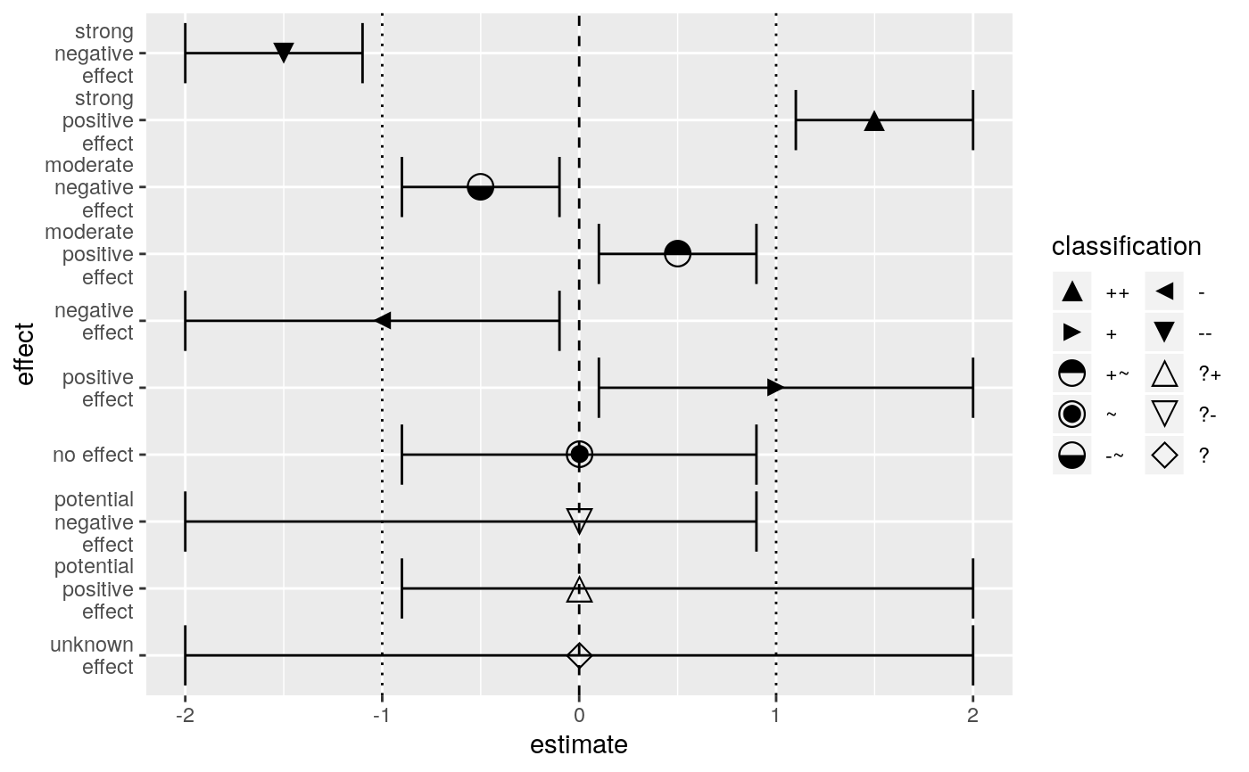
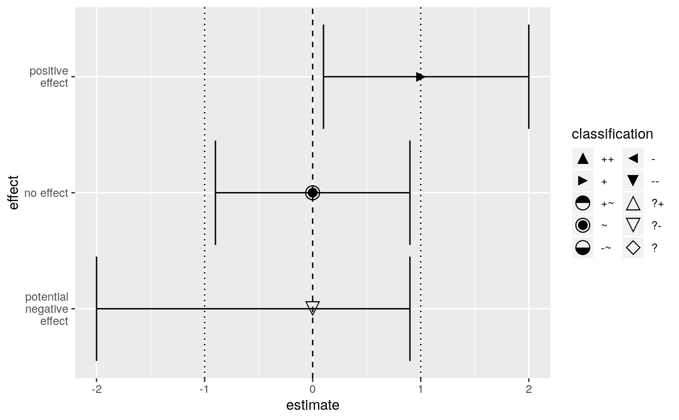
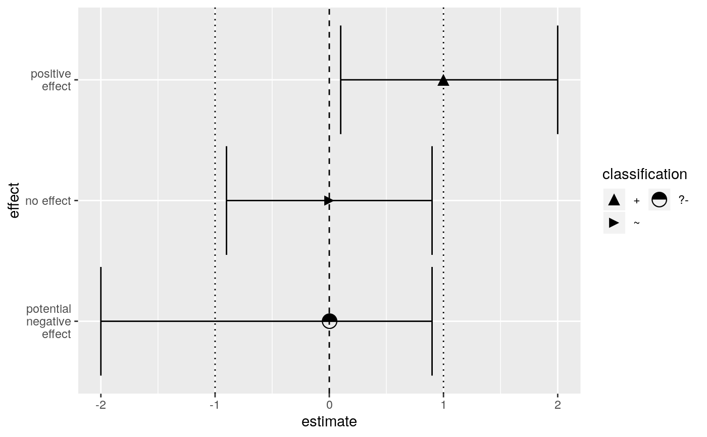
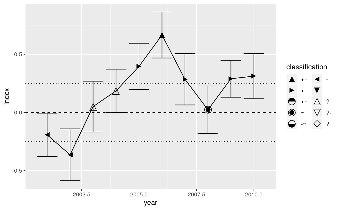
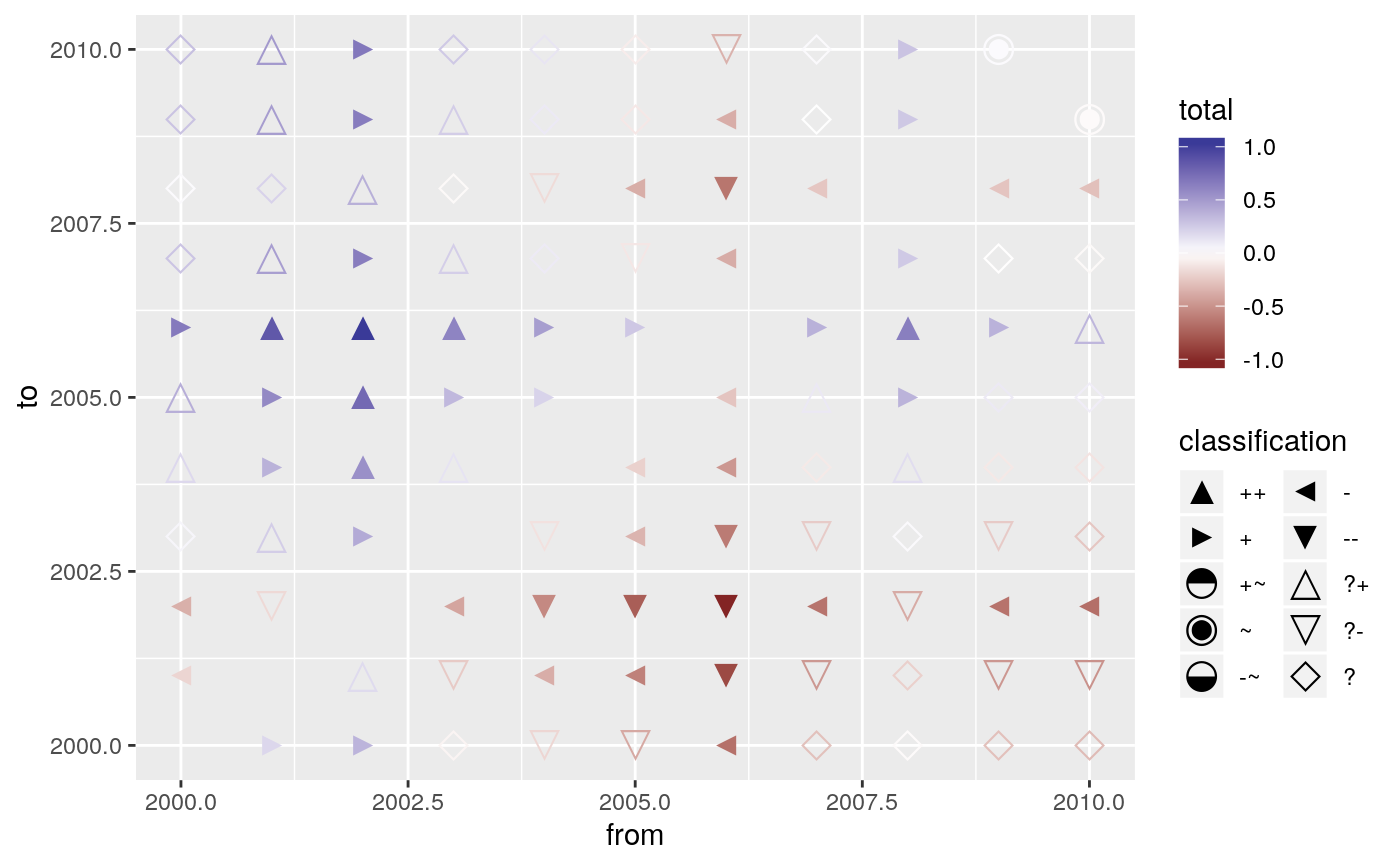
z <- data.frame(
  effect = factor(
    1:10,
    labels = c("unknown\neffect", "potential\npositive\neffect",
             "potential\nnegative\neffect", "no effect", "positive\neffect",
             "negative\neffect", "moderate\npositive\neffect",
             "moderate\nnegative\neffect", "strong\npositive\neffect",
             "strong\nnegative\neffect")
  ),
  estimate = c( 0,  0,    0,   0,   1,   -1,   0.5, -0.5, 1.5, -1.5),
  lcl =      c(-2, -0.9, -2,  -0.9, 0.1, -2,   0.1, -0.9, 1.1, -2),
  ucl =      c( 2,  2,    0.9, 0.9, 2,   -0.1, 0.9, -0.1, 2,   -1.1)
)
oldw <- getOption("warn")
options(warn = -1)
library(ggplot2)
theme_set(theme_grey(base_family = "Helvetica"))
update_geom_defaults("point", list(size = 5))
ggplot(z, aes(x = effect, y = estimate, ymin = lcl, ymax = ucl)) +
  geom_hline(yintercept = c(-1, 1, 0), linetype = c(3, 3, 2)) +
  geom_errorbar() +
  stat_effect(threshold = 1) +
  scale_effect() +
  coord_flip()
ggplot(z[3:5, ], aes(x = effect, y = estimate, ymin = lcl, ymax = ucl)) +
  geom_hline(yintercept = c(-1, 1, 0), linetype = c(3, 3, 2)) +
  geom_errorbar() +
  stat_effect(threshold = 1) +
  scale_effect() +
  coord_flip()
ggplot(z[3:5, ], aes(x = effect, y = estimate, ymin = lcl, ymax = ucl)) +
  geom_hline(yintercept = c(-1, 1, 0), linetype = c(3, 3, 2)) +
  geom_errorbar() +
  stat_effect(threshold = 1) +
  scale_effect(drop = TRUE) +
  coord_flip()

# plot indices
set.seed(20190521)
base_year <- 2000
n_year <- 10
z <- data.frame(
  dt = seq_len(n_year),
  change = rnorm(n_year, sd = 0.2),
  sd = rnorm(n_year, mean = 0.1, sd = 0.01)
)
z$index <- cumsum(z$change)
z$lcl <- qnorm(0.025, z$index, z$sd)
z$ucl <- qnorm(0.975, z$index, z$sd)
z$year <- base_year + z$dt
th <- 0.25
ref <- 0
ggplot(z, aes(x = year, y = index, ymin = lcl, ymax = ucl, sd = sd)) +
  geom_hline(yintercept = c(ref, -th, th), linetype = c(2, 3, 3)) +
  geom_errorbar() +
  geom_line() +
  stat_effect(threshold = th, reference = ref) +
  scale_effect()

# plot pairwise differences
change_set <- function(z, base_year) {
  n_year <- max(z$dt)
  total_change <- lapply(
    seq_len(n_year) - 1,
    function(i) {
      if (i > 0) {
        y <- tail(z, -i)
      } else {
        y <- z
      }
      data.frame(
        from = base_year + i,
        to = base_year + y$dt,
        total = cumsum(y$change),
        sd = sqrt(cumsum(y$sd ^ 2))
      )
    }
  )
  total_change <- do.call(rbind, total_change)
  total_change <- rbind(
    total_change,
    data.frame(
      from = total_change$to,
      to = total_change$from,
      total = -total_change$total,
      sd = total_change$sd
    )
  )
  total_change$lcl <- qnorm(0.025, total_change$total, total_change$sd)
  total_change$ucl <- qnorm(0.975, total_change$total, total_change$sd)
  return(total_change)
}
ggplot(change_set(z, base_year),
       aes(x = from, y = to, ymin = lcl, ymax = ucl)) +
  stat_effect(threshold = th, reference = ref, aes(colour = total)) +
  scale_colour_gradient2() +
  scale_effect()
options(warn = oldw)